🚜 Natural Policy Gradient

🚓 Policy Gradient relies on gradient descent to optimize the policy, which (at least in the world of 🎓 Supervised Learning) is stable and usually converges to some optimum. However, the key issue with simply using gradient descent is that unlike supervised problems that have a fixed data distribution, the data distribution our policy gradient learns from is itself dependent on the policy.

This means that our gradient update step affects the data distribution of our next time step. However, since our gradient was estimated using our current data distribution, it would be inaccurate for a new data distribution that’s different from the current one; that is, if we make a big update to our policy that lands us in a drastically different data distribution, the training process will be unstable.

Theory §

To formalize this problem, we can consider policy gradients as a “soft” version of ♻️ Policy Iteration: rather than directly setting , policy gradients shifts our policy toward that direction via the gradient

In the context of policy iteration, we can view the gradient step as finding some new parameters that maximizes (as that’s the direction of steepest descent).

If we let , we can analytically derive

Observe that maximizing this quantity is the same goal as policy iteration, where we set a new policy that maximizes the advantage calculated by our old policy .

Expanding the right hand side and applying 🪆 Importance Sampling, we have

Unfortunately, the first expectation samples from the distribution defined by , the weights we want to find. This is the formal explanation of our intuitive idea above—the state space is defined by our updated parameters , which we don’t know yet, so a “vanilla” policy gradient step isn’t actually guaranteed to improve at all. Since we only have access to defined by our current policy, the best we can do in this situation is to approximate by bounding the mismatch between and .

Bounding Mismatch §

In order to approximate

we need to bound the difference between and . Since these distributions are determined by our policy, we claim that and are “close” when and are close.

Formally, we define “closeness” between the policies as

where the left hand side is the 👟 Total Variation Distance between the two distributions. It can be shown that given this condition, we can bound

Given this bound on the state distributions, we can then lower bound the true expectation by

where is a constant dependent on the time steps and maximum reward. This result shows that if we optimize this approximation (via vanilla policy gradients), we also maximize our true objective.

Constrained Policy Updates §

Our goal now is to optimize our approximation while ensuring the closeness between our old and new policies. The total variation distance is upper bounded by ✂️ KL Divergence, and we’ll use the KL constraint

for mathematical convenience.

Note that if we compare this constraint with our original policy gradient update, which can be viewed as

our new constraint considers the distributions defined by and rather than the parameters themselves. Intuitively, this accounts for the possibility that a small change in parameter space can cause a big change in probabilities; thus, we’re effectively assigning a small step size for large probability changes and big step size for small probability changes.

The natural policy gradient solves our objective

with the 🌱 Natural Gradient. We first note that the gradient of our objective is

and to find the gradient at our current policy, we plug in to find that

Following the general natural gradient, we approximate our constraint

where is the Fisher-information matrix. The natural policy gradient update is then

where is our Lagrange multiplier. We can manually pick , analogous to the learning rate, or compute it as

if we decide to set from our original KL constraint.

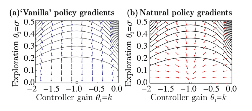
The result of changing the constraint is illustrated below: is our optimal value, and the blue and red arrows are unit directions for the standard and natural policy gradients. We can see that the red arrows are much more direct whereas the blue arrows struggle with converging the axis.