💦 Normalizing Flow

Normalizing flows transform a simple latent distribution into the distribution of a dataset and vice versa. This allows us to sample new images from the dataset distribution and solve other inference problems.

If we could invert and analytically compute , inference wouldn’t require approximation. Normalizing flow’s solution is to use a deterministic and invertible function , so

Note

For invertibility, the dimensions and and must be equivalent.

To transform a random variable’s distribution, we need the change of variables formula

where . Generalizing to vectors, we have

where is the Jacobian with the th row and th column equal to .

A big advantage of this method is that we can now stack transformations on top of each other, as long as they’re all invertible. Hence, we can capture complex distributions be iteratively transforming a simple one.

Variants §

Planar Flow §

Planar flow uses the transformation

where , , and are parameters and is a function of our choice, usually tanh. The determinant of the Jacobian can be computed analytically as

Note that we need to restrict the parameters for the mapping to be invertible, so

NICE §

Nonlinear independence components estimation (NICE) introduces additive coupling layers and rescaling layers. The former are composed together, and the latter is applied at the end.

1. Additive coupling partitions into disjoint subsets and . Then, the corresponding subsets of , and , are equal to the following:

where is a neural network. To invert this, we simply subtract from to recover . 2. Rescaling applies a scaling factor, , with the inverse being its reciprocal.

Note that by design, the Jacobian of the forward mapping for additive coupling is a lower triangular matrix

and the product along the diagonal is . This makes the forward process much more efficient. The Jacobian of the rescaling layer is the product of scaling factors, which is also simple to compute.

Real-NVP §

Real-NVP builds on the additive coupling layer from NICE by adding extra complexity via scaling,

where and are both neural networks. With this form, the Jacobian relies on outputs from , making it more expensive to compute.

Masked Autoregressive Flow §

Masked autoregressive flow (MAF) connects the flow idea to 🕰️ Autoregressive Models that are defined by

If we let the transitions be parameterized Gaussians, we have invertible functions

The Jacobian is lower triangular and can be computed efficiently. However, generation is sequential, taking time.

Inverse Autoregressive Flow §

Inverse autoregressive flow (IAF) addresses the slow generation problem by inverting the neural networks, so we have

where and can now be computed in parallel at the start. Below is a comparison of MAF with IAF.

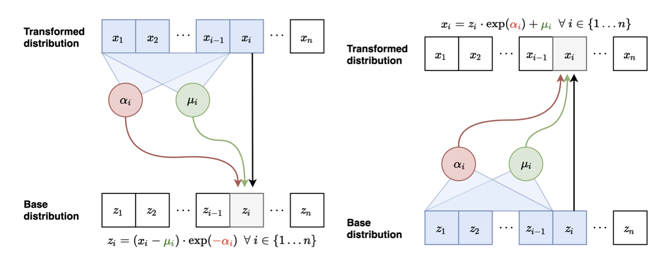
However, the inverse mapping from to is now sequential, making the likelihood evaluation slower.

Parallel Wavenet §

Parallel wavenet combines the best from MAP and IAF speeds by training a teacher and student model. The teacher uses MAF and the student uses IAF. The teacher can be quickly trained via MLE, and the student aims to mimic the teacher by minimizing

Since is generated from the student, its intermediate values can be cached, allowing us to avoid the sequential likelihood calculations.