🗜️ Principle Component Analysis

Principle Component Analysis (PCA) is used for dimensionality reduction, decomposing datapoint vectors in terms of coefficients on orthogonal unit basis vectors . There are infinite bases we can use for , but PCA aims to maximize the variance of the projected points (so that projections don’t collapse points into a single space) and minimize the distortion, or data loss.

Note that we first mean center the data, subtracting from all datapoints. This is used later to relate our equations to covariance, and all operations below will denote as the mean.

Projection §

For an individual vector , its projection onto the basis is defined by

To reconstruct from , we calculate

We can also write this in matrix form; for data arranged in a matrix (such that each row is one vector ),

where containing are the principal component scores and containing are principal components, also called loadings.

Optimization §

We can derive the analytical solution to PCA by following either methodology: minimizing distortion or maximizing variance.

Minimizing Distortion §

Distortion is defined as

Plugging in our definition for and above, we get

This shows that distortion is the sum of squared scores that we leave out. Plugging in the equation for the scores as defined above, we find that distortion actually equals

where is the covariance matrix of our data. (Note that in the equation above, we also swap , but the value remains equivalent.)

To minimize distortion, we first observe that the covariance matrix is symmetric and therefore diagonal in its eigenvector basis. Because it’s diagonal, the axes are independent, and we minimize distortion by leaving out the dimensions that have minimum variance.

Note

For a more mathematical proof, we use Lagrange multipliers. For , to minimize with the constraint that , we differentiate the Lagrangian to get , the definition of an eigenvector.

Setting to be the eigenvectors of the covariance matrix, we see that distortion is the sum of discarded eigenvalues,

Observe that by setting the basis in this way, our basis is orthogonal. In other words, the components are uncorrelated, and the transformation of into gives us uncorrelated features. Moreover, uncorrelated components is intuitively the best way to minimize distortion since any correlation would be redundant.

Maximizing Variance §

Variance is defined as

Note that since we subtract off the mean from , and is excluded from the variance formula above.

Observe that the middle summation is again a form of . The equation then tells us that variance is the sum of squared eigenvalues we do include.

Therefore, by maximizing variance, we’re also minimizing distortion (and vice versa). If we add them together, we get their inverse relationship

Visualization §

As for a visual example, in the image below, we can see that the eigenvectors and their associated eigenvalues (the eigenvector’s magnitude) fit the distortion-minimization variance-maximization objective.

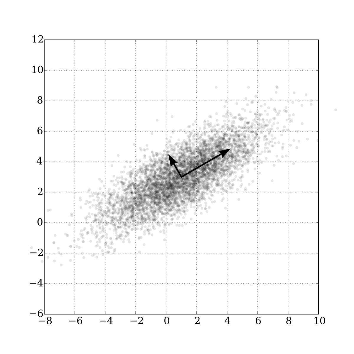
Projecting points onto the largest eigenvector (going from 2D to 1D) will maximize the spread since this axis has largest variance. It also minimizes the distortion, geometrically interpreted as the distance from each point to our new axis.

Computation §

There are two methods to compute the PCA’s eigenvectors. The direct way requires us to find the covariance matrix, which may be computationally expensive; an alternative method uses SVD to avoid this cost.

Direct PCA §

Given data , compute , the average over , and covariance matrix .

Find the largest eigenvalues of and their associated eigenvectors , which are our principal components.

PCA via SVD §

Given data , compute , the average over , and let contains rows .

Compute 📎 Singular Value Decomposition , and take the rows of with the largest singular values as our principal components.

Note that the singular values calculated by SVD for are roots of the eigenvalues of , and the right singular vectors form an orthonormal basis of . The SVD method therefore calculates our eigenvalues and eigenvectors for .

Variants §

PCA has a few variants that add onto its basic functionality.

1. Sparse PCA adds an penalty to the size of the scores and components in our distortion equation, so the optimal values are no longer eigenvectors and require alternating gradient descent.
2. Kernelized PCA can model a nonlinear transformation of the original data.