🕸️ Multilayer Perceptron

Theory §

Multilayer perceptrons, also called feedforward neural networks, can be seen as a non-linear function that outputs some prediction given the input and its learned weights ; in other words, .

As before, we want to minimize the loss , which can be a 📌 Norm for regression or 💧 Cross Entropy for classification.

Neural networks consists of layers of neurons. Each neuron applies weights to its inputs and runs it through an activation function.

Its inputs are the outputs of all neurons in the previous layer, and its output is fed to every neuron in the following layer.

Note

Modern neurons use the ReLU activation function for faster derivative calculation during training and to avoid gradient vanishing (the problem with sigmoid), which leaves the network in weird local minima. Other options include sigmoid and tanh.

A neural network essentially stacks logistic regressions in a complex structure, analogous to pattern recognition. Below is an example of how housing prices could be predicted by a simple network, though it hides links that aren’t used; a proper network should have arrows across all pairs of nodes between two layers.

This is what an actual network looks like.

Regularization §

Some networks incorporate dropout layers, which randomly zero out a fraction of the inputs to the next layer’s neurons, effectively “disconnecting” pairs at random. This provides a regularization effect and pushes networks out of local minima. Note that after training, we use all weights in the network but shrink them by .

Other regularization methods like and in the loss function also apply. applies a weight and gradient clipping effect.

Early stopping is also considered regularization; we prevent overfitting by limiting the amount of iterations our network has to check the training data.

Model §

Neural network model consists of layers of neurons.

Between each neuron in layer and , there is a weight associated with the output of the neuron in that’s inputted into the neuron in .

The first layer’s values are the input features , and final layer is the prediction .

Batch Normalization §

Though a model with only neurons will work fine, batch normalization layers are commonly inserted between them to speed up convergence. This layer normalizes the previous layer’s outputs to have mean zero and unit variance, then scales and shifts it with and , two trainable parameters. This allows the next layer to take in more uniform data, which improves the gradient.

Training §

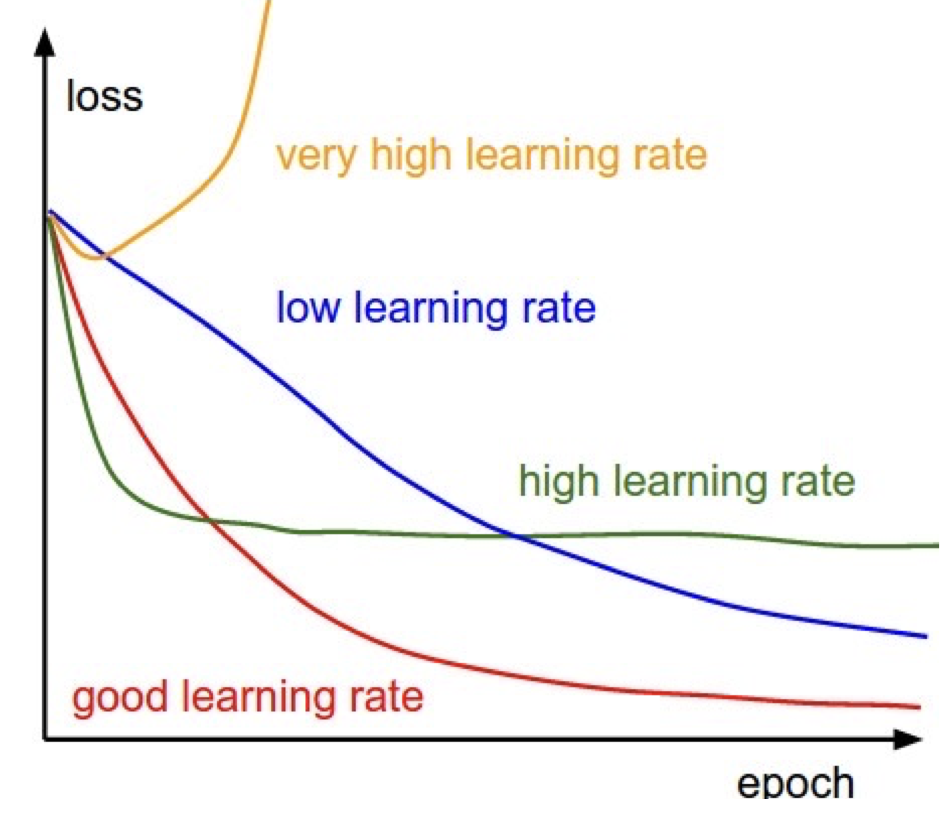
Most commonly trained with ⛰️ Gradient Descent by backpropagating weights using the chain rule, starting from the final layer to the first layer. Choice of learning rate is especially important: if it’s too high, the model can’t converge to a minima; if it’s too low, convergence takes too long.

At each layer, calculate derivatives for each intermediate calculation to find how we should adjust the weights to result in a more accurate prediction.

More advanced optimizers use learning rate adaptation to adjust the learning rate over time; Adagrad increases it for sparse (rare) parameters and decreases it for common ones.

We can also perform feature scaling, ensuring that all features have similar scales, to make gradient descent converge faster.

Finally, transfer learning initializes a model with weights from a previous model trained on a similar dataset. For example, a CNN may use pre-trained weights for its convolutional layers, then only train the dense layers. This essentially initializes the network to already be able to detect small, core patterns, allowing it to converge quicker.

Prediction §

Given input , load features into the first layer of the neural network, then calculate intermediate neuron activations from start to back in a feedforward fashion.