Variational autoencoders are generative models that define an intractable density function using latent variable
Using a similar structure as 🧬 Autoencoders, we use an encoder and decoder to map
Optimization
We choose
The first term can be estimated via 🤔 Monte Carlo Sampling, and the second can be computed analytically since it’s the divergence between two Gaussians. Thus, optimizing the ELBO as a proxy objective with a reconstruction term and a prior regularization term.
Implementation
Concretely, we implement the network as two 👁️ Convolutional Neural Networks. The first predicts
Intuition
We use a probability distribution to force the decoder to recognize that small changes in the sampled latent vector should result in minor changes to the final image. For example, on a single training image, we can have multiple slightly-different sampled latent vectors, and the decoder must learn that they all correspond to the same image.
However, with multiple training examples, it’s still possible for the encoder to generate completely different distributions with low variance and different means, essentially acting as a normal autoencoder. We can mitigate this by regularizing the probability distribution in our loss function, forcing them all to be similar to the standard normal
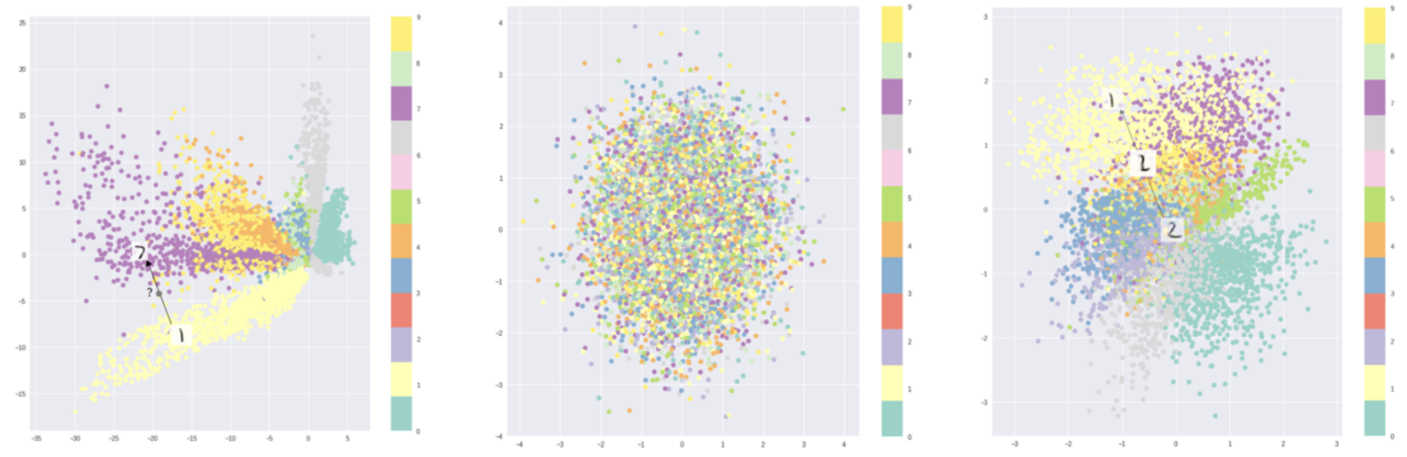
By regularizing the distributions, we force the latent space to be a smooth distribution where any chosen point in the space can be meaningfully reconstructed, as shown in the third graph below.