The contrastive divergence algorithm optimizes the log likelihood of a generative model
The first term is the positive phase, and the second is the negative phase. An intractable positive phase can be solved with approximate inference, but an intractable negative phase is difficult.
Breaking down the negative phase, we can derive
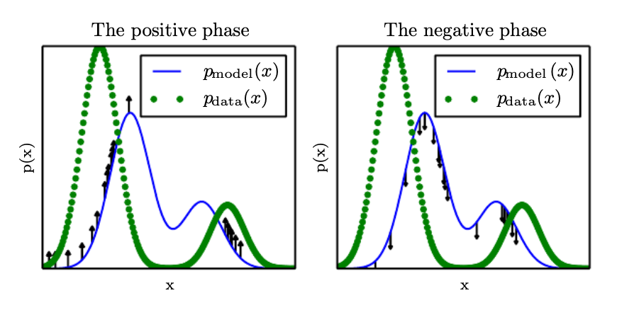
From the above two equations, we can interpret the positive phase as pushing up on the model distribution based on the data and the negative phase as pushing down on the distribution based on our model’s samples. This idea is illustrated below.
There are many ways to implement this gradient update. A naive solution would be to directly estimate the expectation via 🎯 Markov Chain Monte Carlo. However, since burning in the Markov chains is computationally expensive, contrastive divergence initializes the random variables to samples from the actual distribution instead. A single gradient update step is thus the following:
- Sample a minibatch of samples
from the training data. - Compute the positive phase
- Let
for . - For
steps, update with ♻️ Gibbs Sampling. - Compute the negative phase
- Update weights
By initializing the random variables this way, we lose some accuracy in sampling the model distribution. Our negative phase will be extremely inaccurate at the start, but once the positive phase starts shaping the model distribution, the Markov chain will get more accurate.
However, there’s still an issue with this initialization: our random variables will be concentrated in areas where the data distribution is also high. Then, our gradient update won’t suppress the regions of high probability in our model that are far from our data distribution; these areas are called spurious modes.
Persistent Contrastive Divergence
Another way to initialize the random variables is to simply use the values from the previous gradient step. This is based on the assumption that the gradient update is small, so the new model’s distribution stays similar, allowing us to use the already burned-in Markov chains.
This method is called persistent contrastive divergence or stochastic maximum likelihood (SML) in the applied mathematics community.