🖼️ Generative Adversarial Network

GANs are generative models that learn via an adversarial process, which implicitly models the data density function. It consists of a generative and a discriminative network; the former generates samples from a random latent space, and the latter ties to distinguish between generative outputs and samples from the training data.

Specifically, we input random noise into the generator to get an image, and the discriminator predicts the likelihood of real images. Treating this as a two-player game, our minimax objective is

For an optimal discriminator , our objective can be written as

where Jenson-Shannon Divergence

Minimizing this objective is this analogous to making the generator’s distribution close to the data distribution.

For training, we alternate between gradient ascent on slightly-modified parts from the minimax objective:

Challenges §

The above theory, when applied empirically, is often unstable with a few main problems.

1. Unstable optimization and oscillating loss likely caused by imbalance between discriminator and generator effectiveness or oscillation between modes.
2. Generator mode collapse, causing it to generate duplicates consisting of modes of the distribution.

f-GAN §

Instead of using the Jenson-Shannon Divergence, we can generalize the GAN objective to any 🪭 F-Divergence,

for some . However, this is an expectation over only one distribution, and we need to convert it into expectations for both the data and model distributions.

To do this, we use the Fenchel conjugate, defined as

Intuitively, represents linear lower bounds on with slope . Furthermore, it has the property that , so we have

Plugging this into our -divergence, we get the following:

We thus have a lower bound on our objective and can choose any -divergence to optimize. We can parameterize by and the model distribution by to get

which is a generalization of the original GAN objective.

Wasserstein GAN §

The Wasserstein GAN notes that our divergence requires the support of to cover the support of ; if it doesn’t then, there are discontinuities in the divergence function.

To avoid this limitation, we can instead use the Wasserstein distance

where consists of all joint distributions with marginals and . We can interpret as the “earth moving” plan that warps to .

To convert this into two expectations, we use the Kantorovich-Rubinstein duality,

where means the Lipschitz constant of is . Applying the general formula above to our GAN, we get

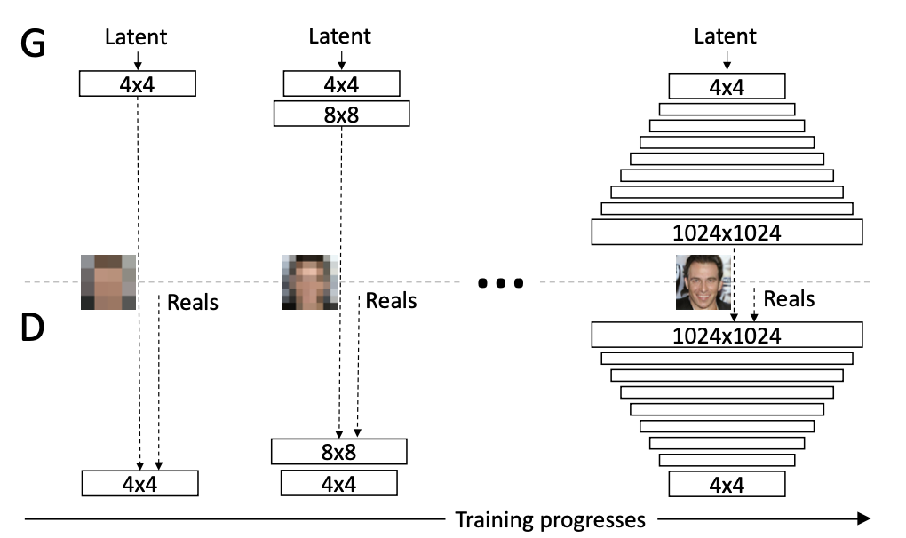
Progressive Growing §

Training instability often arises from the generator and discriminator improving at different levels. To address this problem, we can start by generating small 4x4 resolution images, then slowly scale up the resolution by adding more layers onto the generator and discriminator. This not only encourages faster convergence but also allows the models to see many more images during training due to smaller hardware requirements in the early stages.

BiGAN §

BiGAN infers the latent representation of a sample by training an encoder network along with the generator ; the former maps to and the latter maps to .

Our discriminator objective is to differentiate and . Training adversarially this way allows us to use to move from images to the original noise.