Optical flow finds the visual flow in videos, sort of like 🍿 Two-View Stereopsis but with small baselines. Formally, we wish to compute the positional and angular velocities of the camera,
Local Search
Since the frames of a video are extremely similar, we expect image patches to move very slightly in adjacent frames. Let two adjacent frames be
where
Though this does work in practice, its main weakness is that to search, we discretize
Optimization
Rather than performing an exhaustive search, we can instead frame optical flow as an optimization problem where we want to minimize
The optimal
Since a variation with
and revealing that the fraction is exactly the image gradient of
Taylor Approximation
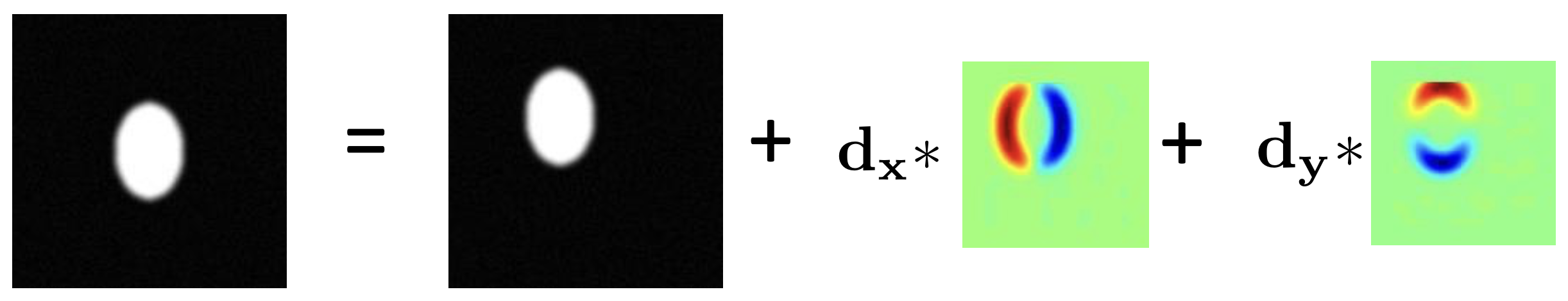
To simplify our task, we can approximate
Visually, this is assuming that the shifted image is the sum of an unshifted version with its gradient, which “shaves” off edges.
Now, our original optimization task turns into
In this form, our problem looks very similar to the least squares problem,
Indeed, we can plug our approximation back into our optimization equation, arriving at
and reordering, we have
exactly mirroring the least squares solution
Another common form of this equation is
The coefficient on the left is the second moment matrix that describes, for each pixel, the second-order gradients. The term on the right is the difference between images, then multiplied with the second image’s gradient. We can compute both terms, and thus we can find
Gradient Descent
However, since we used a Taylor approximation, our first solution for
Windows
Finally, one more thing to note is that we usually perform this optimization over small patches (windows) of an image rather than individual pixels. This objective is
where
and again apply the least squares solution
(Note that
Large Displacements
Our gradient operator
The most direct solution is to use a larger gradient kernel, allowing information to propagate across more pixels and hopefully incorporating parts of the first image. Alternatively, we can use the gaussian pyramid (from 🔺 Image Pyramid) and perform optical flow on smaller images, thereby making the same kernel larger relative to the image.
Texture Challenges
Our approach relies on the assumption that brightness stays similar and the absence of occlusions. We also need the patch to be sufficiently interesting for the left product to be invertible. As such, there are certain scenarios where this algorithm doesn’t work well:
- “White wall” problem: in the absence of texture, we get no gradient and thus no flow.
- “Barber poll” problem: with one-dimensional texture, we get a constant gradient and insufficient information to compute the true flow. This is why the barber pole has an illusion of moving up or down when it’s actually just rotating.
Recovering Velocities
Nevertheless, in the case where we do get
Let
Since
To relate this to calibrated coordinates, we can differentiate the projection equation,
Finally, combining the two equations above allows us to relate the change in calibrated coordinates with
The first term is the translational flow, and the second is the rotational flow that’s independent of depth.
If
Pure Translation
In the case of pure translation, we have the translational flow
and the condition
which says that the image point, flow, and linear velocity lie on the same plane. We can then solve for
via SVD to find the nullspace.
General Case
In the general case where both
where
Rearranging, we have
and for
Our guess for
and then recover both
Time to Collision
One useful thing we can do with optical flow vectors is estimating the time to collision of the camera with something in front of it. Observe that the translational flow
all intersect at a single point—the focus of expansion (FOE). This point can be computed as
The time to collision (TTC) can then be measured as