Usually, it's difficult to directly work with a -th order differential equation model, like those in a ♻️ Transfer Function Model. Thus, a state space model (SSM) expresses it instead as a set of first-order differential equations.

To do so, we introduce new variables called states. For a SISO system with input and output , let the states be

A -th order differential equation

can then be written as

where the final equation comes from rearranging the ODE and substituting states for derivatives of .

These state equations can be summarized in matrix form as

and the output as

More generally, we can represent this as

which is called the state space realization . This is also sometimes written as a single equation via block matrices,

The above SSM is linear (in terms of the derivatives). For a 🇨🇦 Nonlinear State Space Model, we have to make local linear approximations instead.

Solutions#

Let the initial condition be . Then, the solution to a SSM is

This general solution has two parts, called the free response and forced response. The former is the solution with zero input (),

and the latter is the contribution of the input with zero initial condition (),

Free Response#

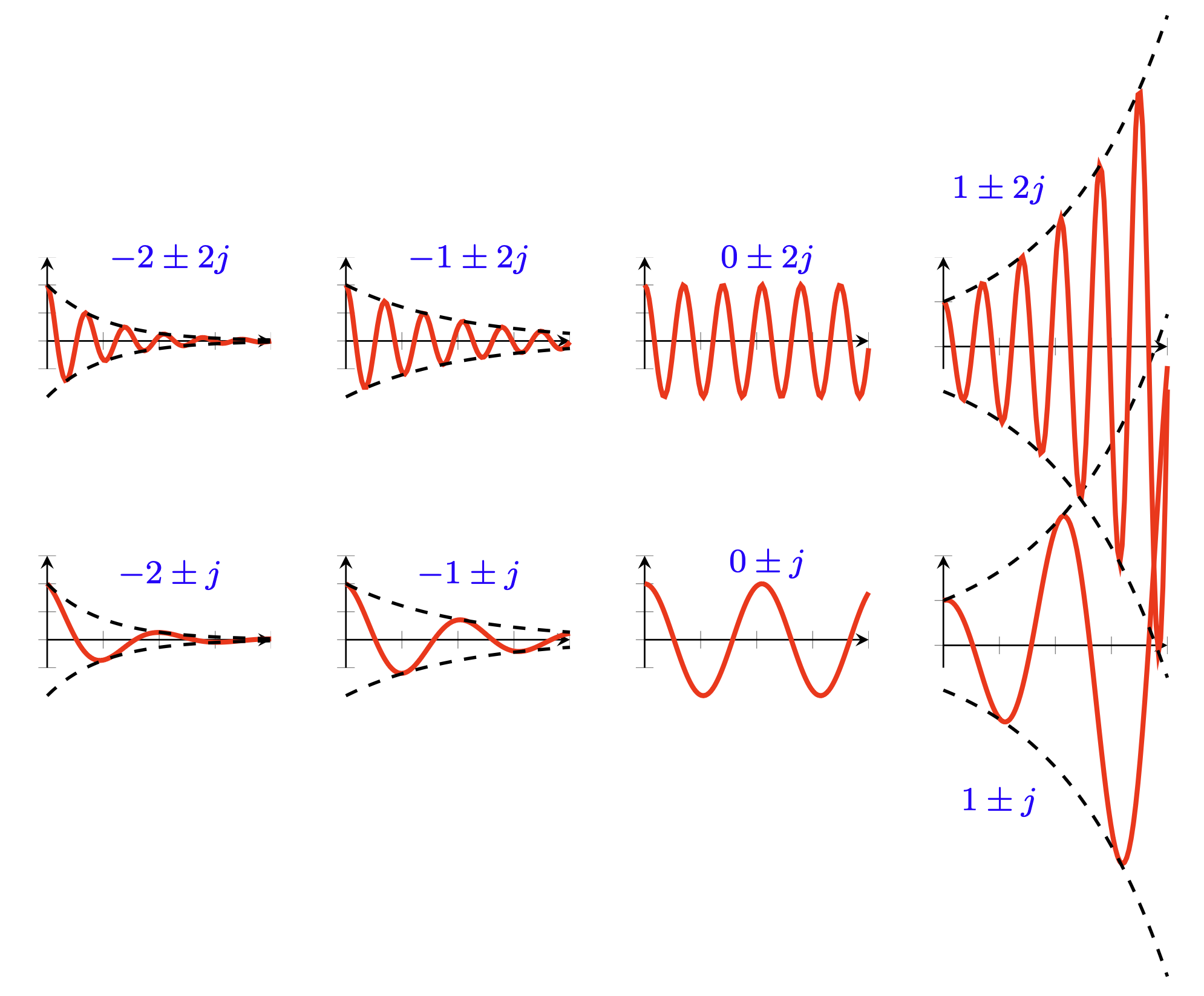
The free response describes how the system behaves without any input. We can analyze the behavior by diagonalizing where has diagonal values . The free response is thus a linear combination of these values, which control how the free response changes over time.

If only has a real term, then it either decays, remains constant, or grows exponentially.

With complex , we have

Thus, the real part controls the magnitude (like above), and the imaginary part introduces oscillations.

State Transition Matrix#

In an unforced system, we can summarize the solution via the state transition matrix , such that

Intuitively, describes how the initial condition transforms into . For an unforced LTI system, we have

For an unforced LTV system, there is no closed form solution. Rather, we can construct the matrix as follows. Let denote the solution of the LTV system when the initial condition , the -th unit vector. Then,

Putting these equations together for , we have

For a forced LTV system, we can still use the state transition matrix, along with a term for the input,