This note is based off the wonderful tutorial at https://huggingface.co/spaces/nanotron/ultrascale-playbook.

Problem#

To scale transformers with hundreds of GPUs, there are 3 key issues:

1. Memory usage: fitting the model and batch into GPU memory.
2. Compute efficiency: spending as much time as possible on computations (instead of data transfer or idling).
3. Communication overhead: minimizing slow communication, parallelizing with compute.

Memory Usage#

Training can be broken down into (1) forward pass to compute prediction, (2) backward pass to compute gradients, and (3) optimization step to update parameters. The information stored in memory include model weights, activations, gradients, and optimizer states.

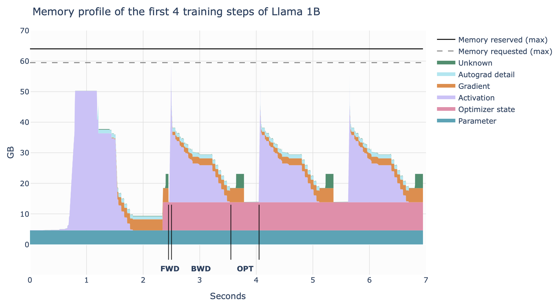
The memory for weights, gradients, and optimizer states depend on the size of the model. For a simple transformer, the number of parameters is

where is the hidden dimension, is vocabulary size, and is number of transformer layers. We have the same number of gradients as parameters, and the Adam optimizer has momentum and variance for each parameter. It's common to see different floating point precisions used here: BF16 for most computations and FP32 for storage. This makes GPU operations faster and reduces activation memory requirements during the forward pass.

Memory for activations is a bit different since it depends on the data batch size. Importantly, it scales linearly with batch size and quadratically with sequence length, so when sequences get longer, it takes up the majority of memory.

Activation Recomputation#

To avoid activation memory from getting too large, activation recomputation will discard some activations during the forward pass and recompute them during the backward pass. Generally, selective recomputation elects to save just the expensive feedforward results and recompute attention on the fly.

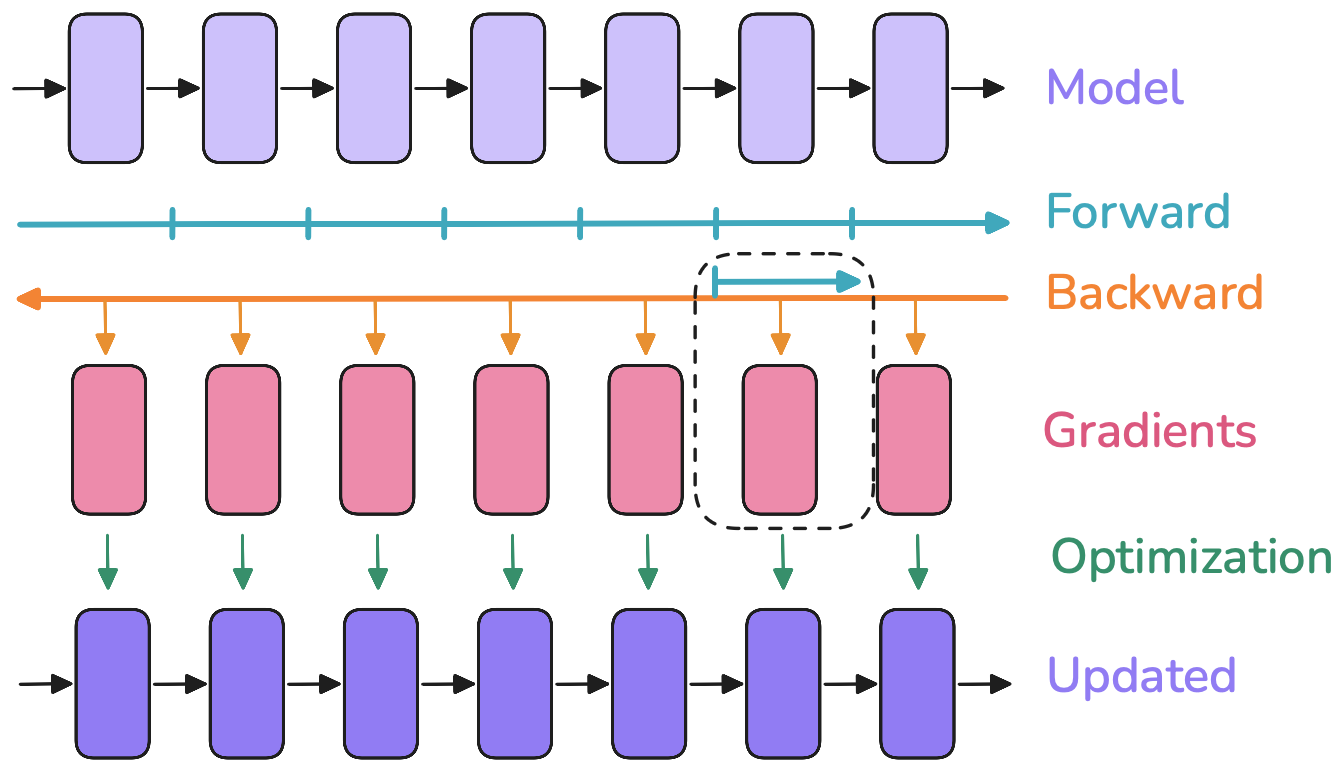
This can often even be faster since accessing memory could be slower than performing computations.

Gradient Accumulation#

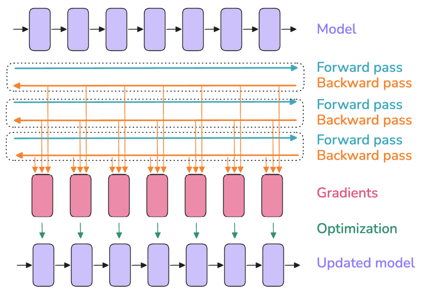
Additionally, we can avoid the linear memory scaling on batch size. Gradient accumulation splits the batch into micro-batches, compute the forward and backward passes independently per micro-batch, then averages the gradients before optimization. However, this naturally increases compute overhead due to multiple forward-backward passes—but this can be parallelized (see below).

Data Parallelism#

With multiple GPUs, the first scaling technique we can use is data parallelism (DP): replicating the model on each GPU and running forward-backward passes on different micro-batches in parallel. Each GPU will then have different gradients, which we average using the all-reduce distributed communication primitive.

Rather than simply waiting for backward passes to finish before all-reduce, there are 3 key optimizations we can make:

1. Overlap gradient synchronization with computation by gathering gradients that have already been computed before we even get to earlier layers.
2. Group gradients into "buckets" and run all-reduce on buckets instead of individual gradients.
3. When coupled with gradient accumulation, run all-reduce only at the final backward pass.

Zero Redundancy Optimizer (ZeRO)#

Data parallelism as described above has a lot of memory redundancy: optimizer states, gradients, and parameters are replicated in each rank. ZeRO instead partitions this information across the data parallel dimension. Note that activations aren't part of this because ranks get different micro-batches and thus different activations.

ZeRO shards the optimizer states, gradients, and parameters across ranks, so memory usage is divided by the data parallel degree.

ZeRO-1 (Optimizer States)#

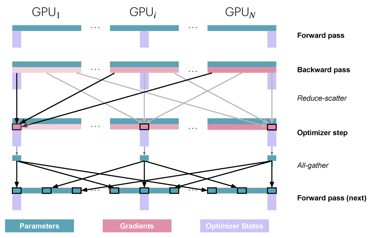
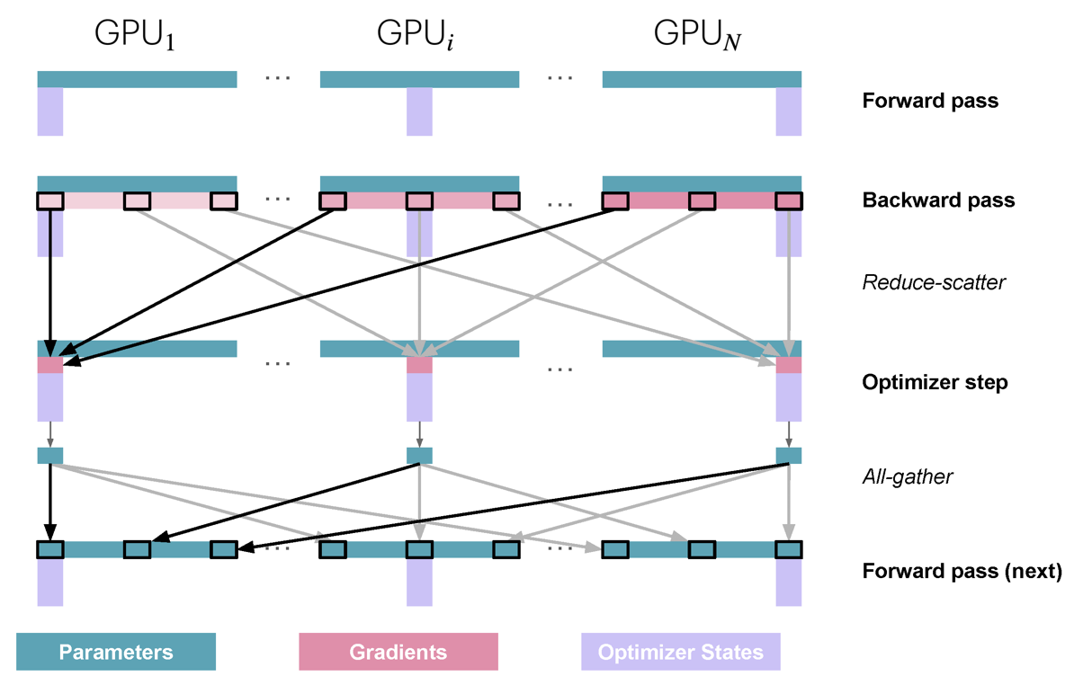
In vanilla DP, all ranks gather the gradients and perform the same optimizer steps. We can avoid this duplicate work by partitioning optimizer steps across ranks; during an optimization step, each rank only updates of its parameters. Then, an all-gather operation ensures that each replica has the full updated parameters.

Before this operation, we collect gradients with a reduce-scatter operation that splits the gradients to their respective ranks.

ZeRO-2 (Optimizer States and Gradients)#

In ZeRO-1, we use the optimizer for only of the updates, so there's no use in having all gradients on all DP ranks. Thus, while we compute all gradients, we give them to reduce-scatter and only store the relevant of results.

ZeRO-3 (Optimizer States, Gradients, and Parameters)#

Now, we can also partition the model parameters. To do a forward or backward pass, we'll run all-gather on the fly whenever we need a set of parameters; the necessary parameters are used and then removed from memory.

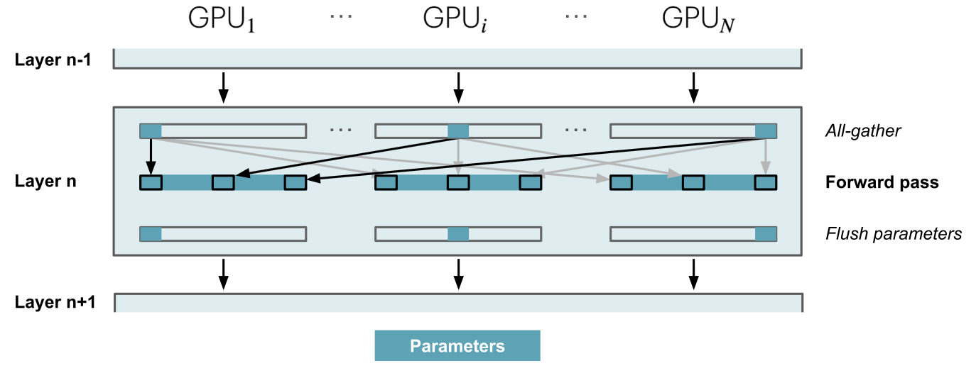
This is a lot of all-gather operations. For optimal efficiency, we can get the weights for layer while running the forward pass for layer (and vice versa for backward pass)—this is called prefetching.

With model parameters, these operations now give us a memory usage of

where is the optimizer multiplier (dependent on optimizer).

Tensor Parallelism#

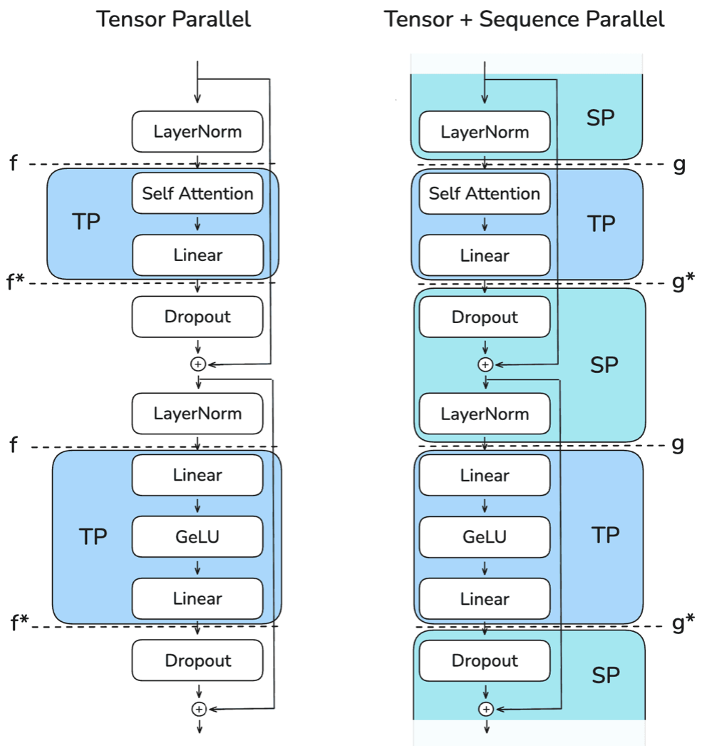
In data parallelism, activation memory is not partitioned. However, this is a bottleneck that scales with sequence length and batch size. Tensor parallelism (TP) proposes to shard activations, along with parameters, gradients, and optimizer states, by exploiting the independence of matrix multiplications:

These equations allow us to compute the product by splitting up : either by column (top) or row (bottom). Transferring this to machine learning, this means we split the weight matrices by column or row. Specifically, for the transformer, we have:

1. In the feedforward MLP, a column-linear followed by a row-linear split on the two weights.
2. In the multi-head attention block, column-linear split on the query/key/value and row-linear split on the output projection.

Naturally, each split goes to a different GPU, reducing the memory needed for parameters, gradients, and optimizer states.

Sequence Parallelism#

A key limitation in the TP formulation above is that some operations like layer normalization and dropout still require the full activations to be present on each GPU. Sequence parallelism (SP) solves this by partitioning along the sequence dimension rather than the hidden (weights) dimension. Combining TP and SP, we alternate between parallelizing across sequence and hidden dimensions.

Context Parallelism#

Although tensor parallelism significantly reduces memory usage, it still operates on the entire sequence and remains limited by sequence length. Context parallelism (CP), similar to sequence parallelism, proposes to split the sequence—this time, in modules where we already apply TP.

Most modules process tokens independently, so this isn't a problem. The only key exception is attention, since each token attends to all other tokens (or the ones before it, for causal attention).

Ring Attention#

To compute attention within CP, we need to communicate all tokens to all GPUs. Ring Attention is a fast way to do so: each GPU alternates between computing attention scores for a shard and sending/receiving another shard. GPUs send these shards in a circular order—hence, "ring" attention.

There a small issue with this setup for causal attention: GPUs responsible for earlier tokens will have less to compute, and thus the compute time is unbalanced. Zig-Zag Ring Attention proposes to mix the order of tokens assigned to GPUs, thus evening out the distribution.

Pipeline Parallelism#

Another potential problem is that if the model itself is too large, exceeding the number of GPUs on a single node (typically 4 or 8), then inter-node communication will slow down the whole pipeline. One more way to reduce the model's memory usage is pipeline parallelism (PP), which splits the layers of a model across GPUs.

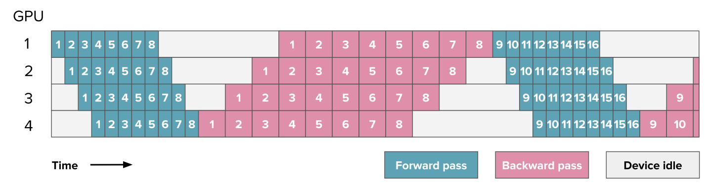
First let's consider splitting the layers in order (so first GPU gets layers , second GPU gets , and so on). Since the forward pass must be run sequentially, this means there's a lot of downtime while some GPUs wait for others to be ready.

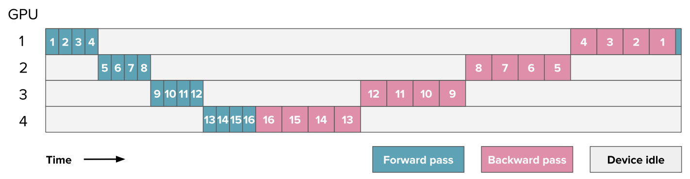
There are a few ways to minimize idle time:

1. All forward, all backward (AFAB): Split the batch into smaller portions, then process them in parallel.
2. One forward, one backward (1F1B): Starting like AFAB, interleave backward passes with forward as soon as possible. This doesn't directly reduce the idle size, but now we only need to store activations for micro-batches ( is degree of parallelism) instead of ( is number of micro-batches), allowing us to have more micro-batches and thus reduce the idle time.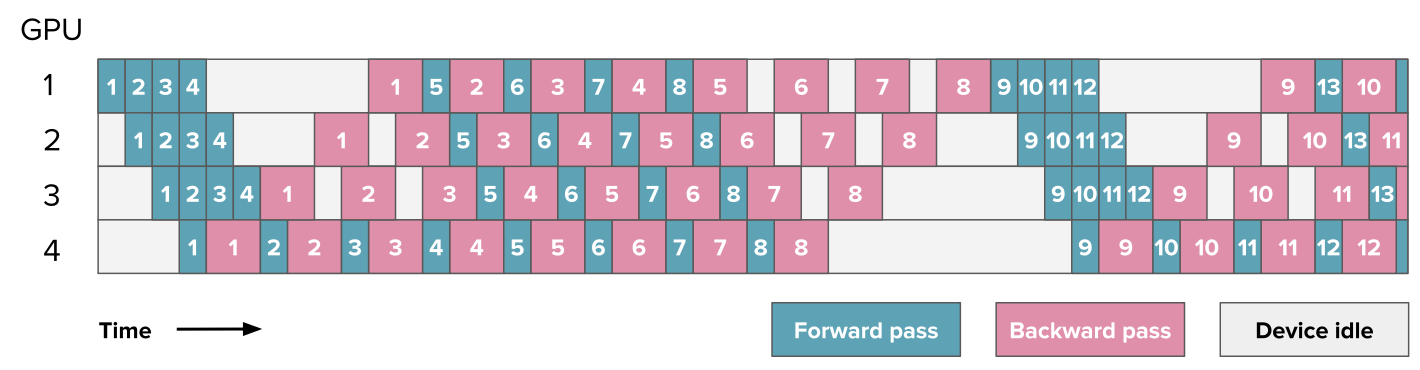
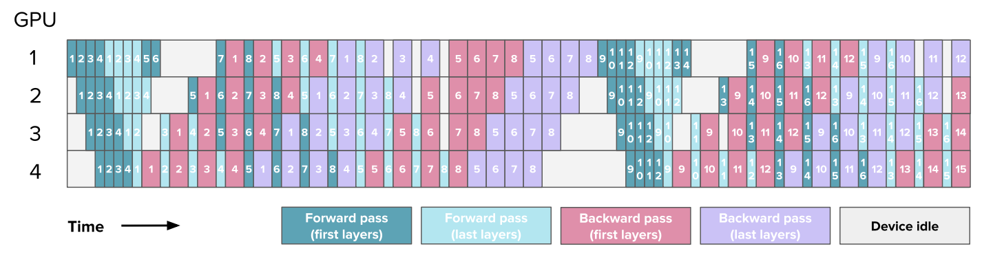
3. Interleaving stages: Instead of splitting layers across GPUs in order, we can interleave layers. Thus allows for even more parallelism.

Expert Parallelism#

Finally, in Mixture of Experts (MoE) models, there are multiple feedforward MLP "experts," and tokens are routed through different experts during inference. Naturally, expert parallelism (EP) puts each expert's feedforward layer on a different worker. This approach is specific just for MoE and thus is often used with other parallelism methods, like DP.