Models with residual connections generally have the form
with hidden layers . We can view this as a discretized transformation of ; in other words, we're changing at discrete time steps with function .
Neural ODEs present a continuous version of this transformation,
where is now continuous, and is now a trainable model with parameters . This is an implicit expression of our solution , which we can solve for using any ODE solver.
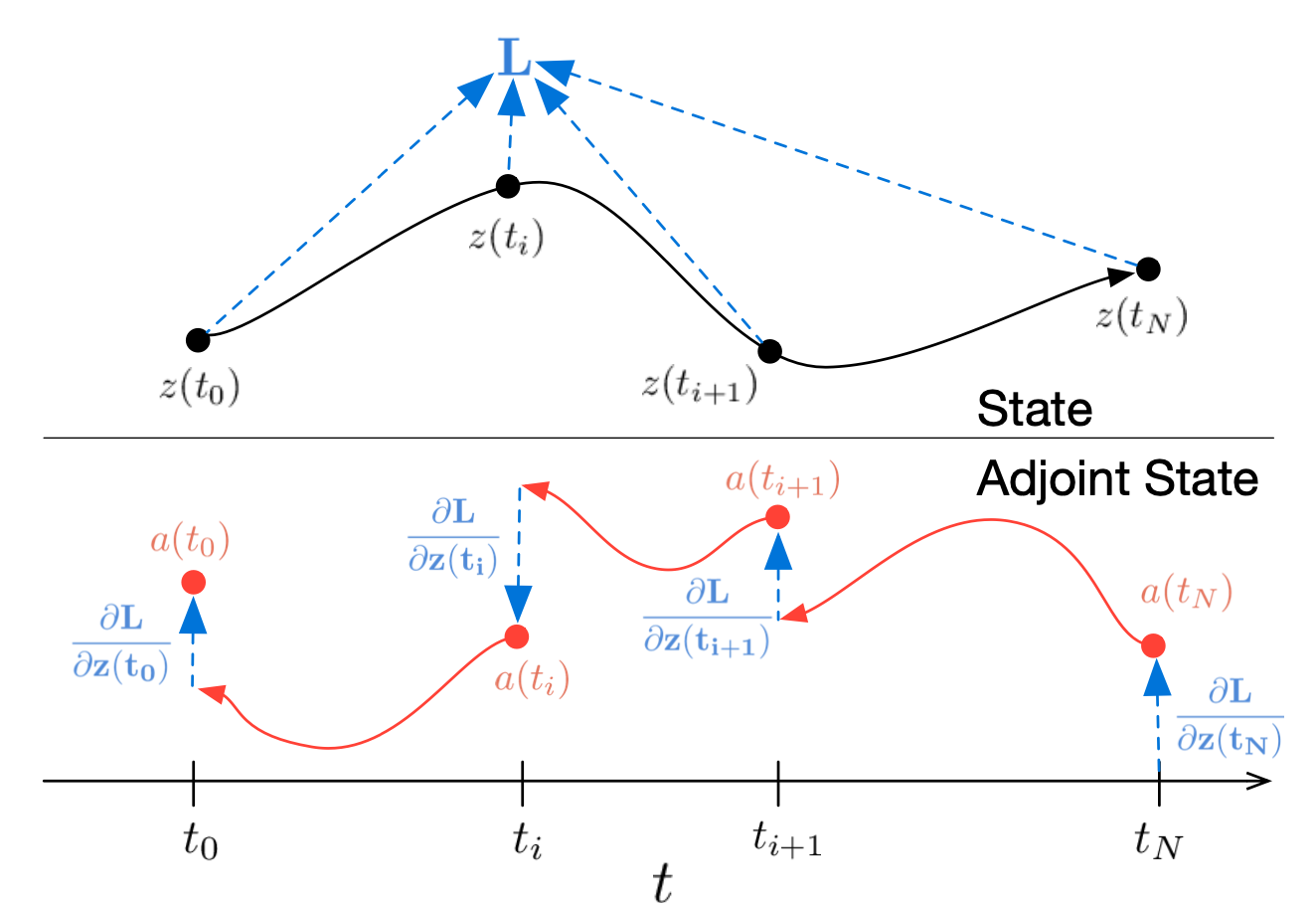
A better interpretation of is not as hidden layers but instead as a hidden variable in a dynamical system. If we let our start time be and end time be , then , defined by the ordinary differential equation above, is our network's prediction. Our goal is thus to minimize the loss
However, computing the gradient isn't as simple as other networks since our loss is now defined by a solution to the ODE, and are the parameters to , not . Instead, we need to first relate the loss with our states ; thus, we first introduce the adjoint
which follows dynamics defined by
We have the value for , so we can find via another call to the ODE solver going backwards from to . Finally, to compute the gradient update, we have
Another common occurrence of the residual connection formula is in 💦 Normalizing Flows with the change of variables formula
where . Applying the same continuous idea to this transformation, we get
This simplifies the normalizing constant to require only a linear computation rather than expensive Jacobian in standard normalizing flows. Experiments have shown that this continuous model is competitive with the standard method.