A dynamical system with state and input is controllable on the interval if for any , there exists that drives the state from to . Here, we'll specifically study controllability for linear systems, in 🇺🇸 State Space Model form, as they have closed-form expressions.
For the state transition
the closed-form solution is
where is the state transition matrix. Controllability is thus the ability to find such that
and are arbitrary, so the RHS must be able to match any vector in .
In other words, if we view as an input and the remaining RHS as an operator, this means its range is . Defining the operator as
we can first multiply it with since is invertible, so the range doesn't change. Then, multiplying with , we have
Using the property of 🍱 Matrix > Adjoints, the range of operator is the same as that of the matrix
We call the controllability Grammian. In summary, a linear system is controllable if this controllability Grammian is full rank.
For something more concrete, we focus on LTI systems, where the state transition matrix
Plugging this into the controllability Grammian, we have
While this still has a somewhat complex form, its range is actually the same as that of
which we call the controllability matrix. Intuitively, this is because expanding gives us terms, and integrating simply makes combinations of these terms. Thus, we conclude that the system is controllable if this has full rank.
In the case of a system in controllable canonical form, the controllability matrix becomes
and is thus full rank. Additionally, the controllability matrix is related to the transformation from system to controllable canonical form (above). Defining transformation
we have
After this transformation, assigning eigenvalues can be done via the procedure above, giving us . Then, we can recover for the original system via
This works because , meaning and are related by similar transform and thus share the same eigenvalues.
Note that in more simple cases, transforming the system into controllable canonical form may not be necessary; it's possible to directly solve for by writing out the characteristic polynomial of and equating it with .
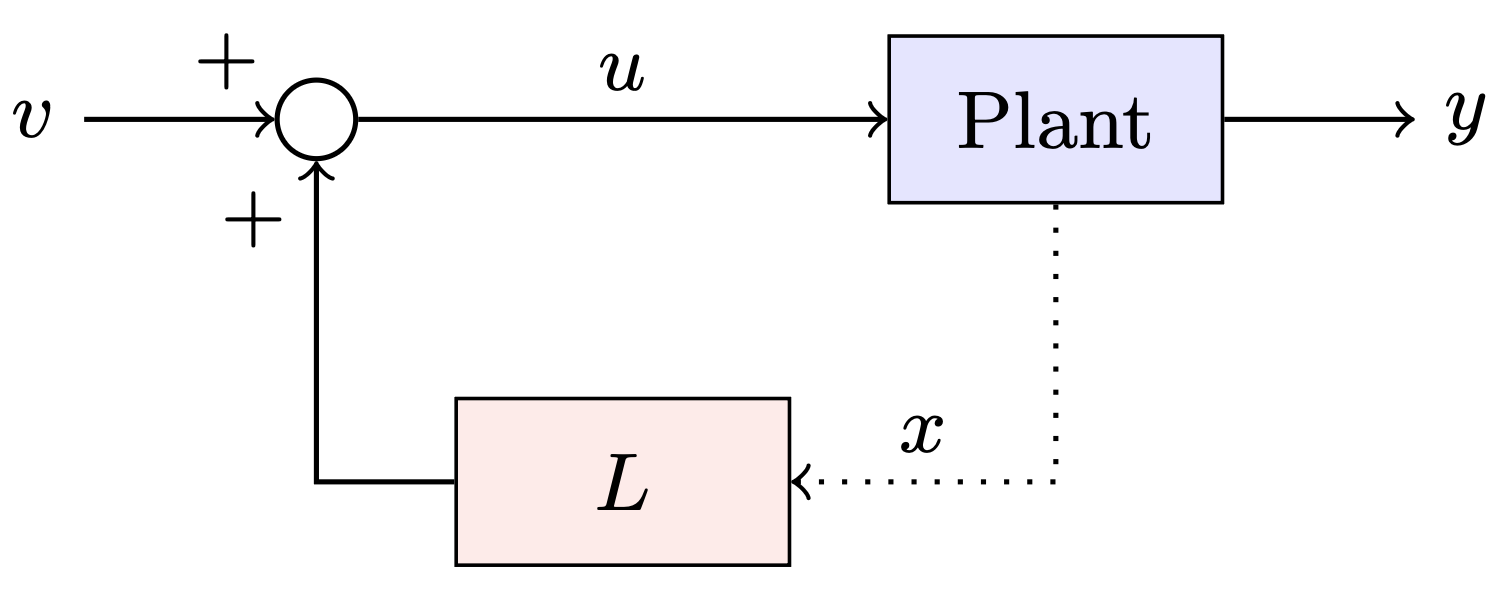
is controllable, we can choose input so reach desired states. This allows us to control the behavior of the system, and especially its stability (see 🇺🇸 State Space Model > Free Response), via the state feedback connection
where is the new input and is computed based on system state .
Now, our whole closed-loop system has
Notice that now our system behavior is decided by the eigenvalues of , and we can choose as we wish to place the eigenvalues of .
We can convert any single-input system to controllable canonical form. We compute
and define as
Note that not all systems can be put into controllable canonical form, and thus not all systems are controllable. In other cases, some eigenvalues may not be expressed in terms of .
For multi-input systems , Heymann's lemma states that for such that , there exists a matrix such that the single-input system is controllable.
This allows us to place eigenvalues for multi-input systems as follows. Pick and let be from Heymann's lemma, and treat as a single-input system; using the above techniques, we can find such that has the desired eigenvalues, then rearrange
to find that gives us desired eigenvalues for the original .
If a system is uncontrollable, we can use 🖖 Kalman Decomposition. This gives us the similarity transform such that
where and are controllable. Then, adding the feedback connection gives us
and splitting into , we have
This tells us that the eigenvalues of are those of and , where the former can be assigned to our desired values and the latter cannot. From this, we note that even if a system is uncontrollable, it can be stable if the uncontrollable portion does not diverge. Such a system is called stabilizable: if there exists such that is stable, where uncontrollable eigenvalues have negative real parts.
Finally, we can assess the responsiveness of different state directions to the input—that is, how easily different states can be controlled. To do so, we'll first study what states we can reach, going from time to with constrained inputs , . These states are described via
If we further restrict to , the reachable set of states remains unchanged (since the lost inputs are part of null space and go to zero). This equivalently means , so we can define as
which means
where is the controllability Grammian described above. In addition, the magnitude constraint on enforces
Therefore, we can see that the reachable set of states is defined by the controllability Grammian. In fact, this set is an ellipsoid, where axes are determined by eigenvectors of , each with length determined by associated eigenvalues. Thus, shows the directions in state space where the system is most responsive to inputs: directions with larger eigenvalues are much easier to control.